Choose your fighter

In order to apply bayesian inference to real world problems, you need to pick a Probabilistic Programming Language (PPL) to express your models as code. There are a number to choose from, and each one has a specific backend that you might need to understand if you need to debug your code.

Why are backends important?

Most Probabilistic Programming Languages (PPLs) in Python are powered by a tensor library under the hood, and this choice can greatly alter your experience. I didn’t come from a deep learning background, but some of the lower level frameworks (pyro, tensorflow probability) use these deep learning frameworks as a backend so at least surface-level understanding with these libraries will be needed when you need to debug your code and help you read others’ code.

This is just to say that knowing PyTorch or Tensorflow will be helpful to you and point you towards a specific language, but if you don’t know either of these then you’ll need to pick the one that looks better to you. If you had a lot of free time you could learn multiple PPLs and frameworks to see which one you prefer, but like any programming language it’s best to just pick one to start and become productive with it before moving on to another language.

PPL	Backend
pymc	pytensor
pyro	pytorch
numpyro	JAX
pystan	stan
tensorflow probability	tensorflow, keras, JAX

We can look at the github star histories too to see what seems to be more popular:

At the time of this writing, pymc and pyro are the two leading PPLs (in terms of github stars) but anecdotally I think you’ll find a lot more resources around pymc when it comes to examples.

Comparing PPLs wth a simple regression model

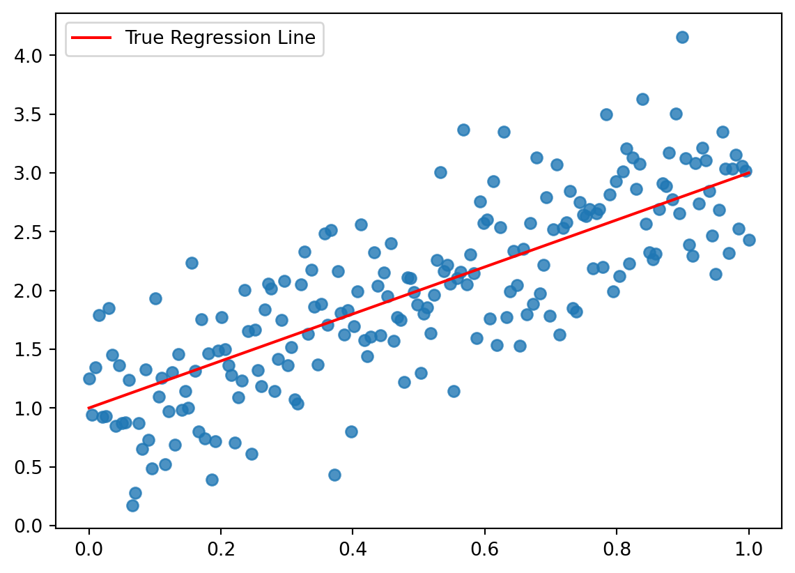
Below we’ll use some examples from pymc, pyro, numpyro, and pystan each fitting a linear regression model so you can look at the syntax. The model is as follows:

\[ \begin{aligned} \text{intercept} &\sim \operatorname{Normal}(0, 20)\\ \text{slope} &\sim \operatorname{Normal}(0, 20)\\ \text{sigma} &\sim \operatorname{HalfCauchy}(10)\\ \mu &= \text{intercept} + \text{slope} * x \\ y &\sim \operatorname{Normal}(\mu, \sigma) \end{aligned} \]

The graph representation of this model (i.e. Plate Notation) is:

Model Rendering

The dark circle represents the observed variable \(y\) and the variables in white are latent or unobserved variables that we wish to infer.

Code

The following code will try to infer the hidden parameters from some synthetic data where the true parameters are:

Intercept = 1
Slope = 2
Sigma = 0.5

See below for sample code to generate the synthetic data.

import arviz as az
import pandas as pd
import matplotlib.pyplot as plt
import numpy as np

# Simulate Data
np.random.seed(42)

size = 200
true_intercept = 1
true_slope = 2
true_sigma = 0.5

x = np.linspace(0, 1, size)
# y = a + b*x
true_regression_line = true_intercept + true_slope * x
# add noise
y = true_regression_line + np.random.normal(0, true_sigma, size)

plt.scatter(x, y, alpha=0.8)
plt.plot(x, true_regression_line, c="r", label="True Regression Line")
plt.legend();

pymc has undergone many changes but remains the easiest path for pythonistas to start building and running models.

import pymc as pm

# model specifications in PyMC are wrapped in a with-statement
with pm.Model() as pymc_model:
    # Define priors
    sigma = pm.HalfCauchy("sigma", beta=10)
    intercept = pm.Normal("Intercept", 0, sigma=20)
    slope = pm.Normal("slope", 0, sigma=20)

    # Define likelihood
    mu = intercept + slope * x
    likelihood = pm.Normal("y", mu=mu, sigma=sigma, observed=y)

WARNING (pytensor.tensor.blas): Using NumPy C-API based implementation for BLAS functions.

Inference is as simple as calling the pm.sample() function within the model context. pymc also offers additional samplers such as blackjax and numpyro that may be more performant than the default backend.

with pymc_model:
    # draw 1000 posterior samples using NUTS and the numpyro backend
    idata = pm.sample(1000, nuts_sampler="numpyro", chains=2)

	mean	sd	hdi_3%	hdi_97%	mcse_mean	mcse_sd	ess_bulk	ess_tail	r_hat
Intercept	0.921	0.068	0.794	1.046	0.003	0.002	651.0	859.0	1.00
sigma	0.467	0.024	0.424	0.513	0.001	0.001	1075.0	1005.0	1.01
slope	2.118	0.119	1.908	2.356	0.005	0.003	652.0	739.0	1.00

import pyro
import pyro.distributions as dist
import torch


def pyro_model(x, y=None):
    # Convert the data from numpy array to torch tensors
    x = torch.tensor(x)
    if y is not None:
        y = torch.tensor(y)

    # Model specification
    sigma = pyro.sample("sigma", dist.HalfCauchy(10))
    intercept = pyro.sample("intercept", dist.Normal(0, 20))
    slope = pyro.sample("slope", dist.Normal(0, 20))

    mu = intercept + slope * x

    # likelihood
    pyro.sample("y", dist.Normal(mu, sigma), obs=y)

If this were pymc, we’d be done by now! Here, we need to add some extra steps to perform inference while pymc tries to be more ‘batteries included’.

from pyro.infer import MCMC, NUTS

nuts_kernel = NUTS(pyro_model)
pyro_mcmc = MCMC(kernel=nuts_kernel, warmup_steps=1000, num_samples=1000, num_chains=2)
# Run with model args
pyro_mcmc.run(x, y)

/home/nelsont/.cache/pypoetry/virtualenvs/banditkings-fWuXf1Do-py3.10/lib/python3.10/site-packages/arviz/data/io_pyro.py:158: UserWarning:

Could not get vectorized trace, log_likelihood group will be omitted. Check your model vectorization or set log_likelihood=False

	mean	sd	hdi_3%	hdi_97%	mcse_mean	mcse_sd	ess_bulk	ess_tail	r_hat
intercept	0.922	0.066	0.801	1.046	0.002	0.002	733.0	937.0	1.0
sigma	0.468	0.023	0.427	0.511	0.001	0.001	1022.0	1170.0	1.0
slope	2.113	0.115	1.911	2.333	0.004	0.003	761.0	993.0	1.0

numpyro shares many similarities with pyro but uses a faster jax backend and offers significant performance improvements over pyro. The downside is that numpyro is still under active development and may be missing a lot of functionality that pyro users have.

# Modeling
import numpyro
import numpyro.distributions as dist
from jax import random
import jax.numpy as jnp
from numpyro.infer import MCMC, NUTS


# Model specifications in numpyro are in the form of a function
def numpyro_model(x, y=None):
    sigma = numpyro.sample("sigma", dist.HalfCauchy(10))
    intercept = numpyro.sample("Intercept", dist.Normal(0, 20))
    slope = numpyro.sample("slope", dist.Normal(0, 20))

    # define likelihood
    mu = intercept + slope * x
    likelihood = numpyro.sample("y", dist.Normal(mu, sigma), obs=y)

    return likelihood

Inference in numpyro is similar to pyro, with the exception of the added step to set the jax pseudo-random number generator key.

# Inference
nuts_kernel = NUTS(numpyro_model)
mcmc = MCMC(nuts_kernel, num_chains=2, num_warmup=1000, num_samples=1000)

# JAX needs an explicit pseudo-random number generator key
rng_key = random.PRNGKey(seed=42)
# Finally, run our sampler
mcmc.run(rng_key, x=x, y=y)

	mean	sd	hdi_3%	hdi_97%	mcse_mean	mcse_sd	ess_bulk	ess_tail	r_hat
Intercept	0.926	0.064	0.801	1.045	0.002	0.002	830.0	1070.0	1.0
sigma	0.468	0.023	0.425	0.512	0.001	0.001	995.0	899.0	1.0
slope	2.108	0.111	1.883	2.301	0.004	0.003	820.0	1145.0	1.0

PyStan offers a python interface to stan on Linux or macOS (windows user can use WSL). PyStan 3 is a complete rewrite from PyStan 2 so be careful with using legacy code. The following uses PyStan 3.10.

import stan

# NOTE: Running pystan in jupyter requires nest_asyncio
import nest_asyncio

nest_asyncio.apply()

# Let's silence some warnings
import logging

# silence logger, there are better ways to do this
# see PyStan docs
logging.getLogger("pystan").propagate = False

stan_model = """
data {
  int<lower=0> N;
  vector[N] x;
  vector[N] y;
}
parameters {
  real intercept;
  real slope;
  real<lower=0> sigma;
}
model {
  // priors
  intercept ~ normal(0, 20);
  slope ~ normal(0, 20);
  sigma ~ cauchy(0, 10);
  // likelihood
  y ~ normal(intercept + slope * x, sigma);
}
"""

data = {"N": len(x), "x": x, "y": y}

# Build the model in stan
posterior = stan.build(stan_model, data=data, random_seed=1)

# Inference/Draw samples
posterior_samples = posterior.sample(num_chains=2, num_samples=1000)

The result is a stan.fit.Fit object that you can run through arviz with az.summary().

	mean	sd	hdi_3%	hdi_97%	mcse_mean	mcse_sd	ess_bulk	ess_tail	r_hat
intercept	0.921	0.065	0.800	1.039	0.002	0.002	919.0	1071.0	1.0
sigma	0.467	0.023	0.421	0.508	0.001	0.001	828.0	1050.0	1.0
slope	2.116	0.113	1.913	2.324	0.004	0.003	902.0	1066.0	1.0

Final Thoughts

I started with pymc for initial concepts and as a first pass, but I quickly hit a point where I needed the flexibility of a lower level language to do the kinds of modeling that I want to do. The numpy-esque syntax of the JAX backend behind numpyro seemed most appealing to me and that’s the path that I’m on.